LU decomposition

In linear algebra, LU decomposition (also called LU factorization) is a matrix decomposition which writes a matrix as the product of a lower triangular matrix and an upper triangular matrix. The product sometimes includes a permutation matrix as well. This decomposition is used in numerical analysis to solve systems of linear equations or calculate the determinant of a matrix. LU decomposition can be viewed as a matrix form of Gaussian elimination. LU decomposition was introduced by mathematician Alan Turing ^[1]

1 Definitions
2 Existence and uniqueness
3 Positive definite matrices
4 Explicit formulation
5 Algorithms
6 Small example
7 Sparse matrix decomposition
8 Applications
9 See also
10 References
11 External links

Definitions

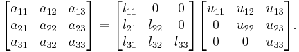
Let A be a square matrix. An LU decomposition is a decomposition of the form

$A = LU, \,$

where L and U are lower and upper triangular matrices (of the same size), respectively. This means that L has only zeros above the diagonal and U has only zeros below the diagonal. For a $3 \times 3$ matrix, this becomes:

$\begin{bmatrix} a_{11} & a_{12} & a_{13} \\ a_{21} & a_{22} & a_{23} \\ a_{31} & a_{32} & a_{33} \\ \end{bmatrix} = \begin{bmatrix} l_{11} & 0 & 0 \\ l_{21} & l_{22} & 0 \\ l_{31} & l_{32} & l_{33} \\ \end{bmatrix} \begin{bmatrix} u_{11} & u_{12} & u_{13} \\ 0 & u_{22} & u_{23} \\ 0 & 0 & u_{33} \\ \end{bmatrix}.$

An LDU decomposition is a decomposition of the form

$A = LDU, \,$

where D is a diagonal matrix and L and U are unit triangular matrices, meaning that all the entries on the diagonals of L and U are one.

An LUP decomposition (also called a LU decomposition with partial pivoting) is a decomposition of the form

$PA = LU, \,$

where L and U are again lower and upper triangular matrices and P is a permutation matrix, i.e., a matrix of zeros and ones that has exactly one entry 1 in each row and column.

An LU decomposition with full pivoting (Trefethen and Bau) takes the form

$PAQ = LU, \,$

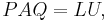
Above we required that A be a square matrix, but these decompositions can all be generalized to rectangular matrices as well. In that case, L and P are square matrices which each have the same number of rows as A, while U is exactly the same shape as A. Upper triangular should be interpreted as having only zero entries below the main diagonal, which starts at the upper left corner.

Existence and uniqueness

An invertible matrix admits an LU factorization if and only if all its leading principal minors are non-zero. The factorization is unique if we require that the diagonal of L (or U) consist of ones. The matrix has a unique LDU factorization under the same conditions.

If the matrix is singular, then an LU factorization may still exist. In fact, a square matrix of rank k has an LU factorization if the first k leading principal minors are non-zero, although the converse is not true.

The exact necessary and sufficient conditions under which a not necessarily invertible matrix over any field has an LU factorization are known. The conditions are expressed in terms of the ranks of certain submatrices. The Gaussian elimination algorithm for obtaining LU decomposition has also been extended to this most general case (Okunev & Johnson 1997).

Every invertible matrix A admits an LUP factorization.

Positive definite matrices

If the matrix A is Hermitian and positive definite, then we can arrange matters so that U is the conjugate transpose of L. In this case, we have written A as

$A = L L^{*}. \,$

This decomposition is called the Cholesky decomposition. The Cholesky decomposition always exists and is unique. Furthermore, computing the Cholesky decomposition is more efficient and numerically more stable than computing some other LU decompositions.

Explicit formulation

When an LDU factorization exists and is unique there is a closed (explicit) formula for the elements of L, D, and U in terms of ratios of determinants of certain submatrices of the original matrix A (Householder 1975). In particular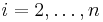, $D_1 = A_{1,1}$ and for $i = 2, \ldots, n$ , $D_i$ is the ratio of the $i^{th}$ principal submatrix to the $(i-1)^{th}$ principal submatrix.

Algorithms

The LU decomposition is basically a modified form of Gaussian elimination. We transform the matrix A into an upper triangular matrix U by eliminating the entries below the main diagonal. The Doolittle algorithm does the elimination column by column starting from the left, by multiplying A to the left with atomic lower triangular matrices. It results in a unit lower triangular matrix and an upper triangular matrix. The Crout algorithm is slightly different and constructs a lower triangular matrix and a unit upper triangular matrix.

Computing the LU decomposition using either of these algorithms requires 2n³ / 3 floating point operations, ignoring lower order terms. Partial pivoting adds only a quadratic term; this is not the case for full pivoting.^[2]

Doolittle algorithm

Given an N × N matrix

$A= (a_{n,n})$

we define

$A^{(0)}�:= A$

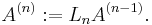
and then we iterate n = 1,...,N-1 as follows.

We eliminate the matrix elements below the main diagonal in the n-th column of A^(n-1) by adding to the i-th row of this matrix the n-th row multiplied by

$l_{i,n}�:= -\frac{a_{i,n}^{(n-1)}}{a_{n,n}^{(n-1)}}$

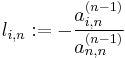
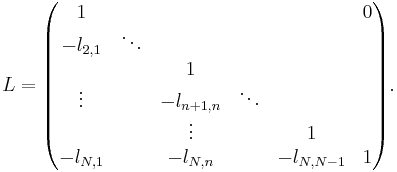
for 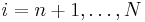$i = n%2B1,\ldots,N$ . This can be done by multiplying A^(n-1) to the left with the lower triangular matrix

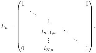
$L_n = \begin{pmatrix} 1 & & & & & 0 \\ & \ddots & & & & \\ & & 1 & & & \\ & & l_{n%2B1,n} & \ddots & & \\ & & \vdots & & \ddots & \\ 0 & & l_{N,n} & & & 1 \\ \end{pmatrix}.$

We set

$A^{(n)}�:= L_n A^{(n-1)}.$

After N-1 steps, we eliminated all the matrix elements below the main diagonal, so we obtain an upper triangular matrix A^(N-1). We find the decomposition

$A = L_{1}^{-1} L_{1} A^{(0)} = L_{1}^{-1} A^{(1)} = L_{1}^{-1} L_{2}^{-1} L_{2} A^{(1)} = L_{1}^{-1}L_{2}^{-1} A^{(2)} =\ldots = L_{1}^{-1} \ldots L_{N-1}^{-1} A^{(N-1)}.$

Denote the upper triangular matrix A^(N-1) by U, and 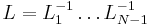$L=L_{1}^{-1} \ldots L_{N-1}^{-1}$ . Because the inverse of a lower triangular matrix L_n is again a lower triangular matrix, and the multiplication of two lower triangular matrices is again a lower triangular matrix, it follows that L is a lower triangular matrix. Moreover, it can be seen that

$L = \begin{pmatrix} 1 & & & & & 0 \\ -l_{2,1} & \ddots & & & & \\ & & 1 & & & \\ \vdots & & -l_{n%2B1,n} & \ddots & & \\ & & \vdots & & 1 & \\ -l_{N,1} & & -l_{N,n} & & -l_{N,N-1} & 1 \\ \end{pmatrix}.$

We obtain $A=LU$ .

It is clear that in order for this algorithm to work, one needs to have $a_{n,n}^{(n-1)}\not=0$ at each step (see the definition of $l_{i,n}$ ). If this assumption fails at some point, one needs to interchange n-th row with another row below it before continuing. This is why the LU decomposition in general looks like $P^{-1}A = L U$ .

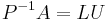Crout and LUP algorithms

The LUP decomposition algorithm by Cormen et al. generalizes Crout matrix decomposition. It can be described as follows.

If $A$ has a nonzero entry in its first row, then take a permutation matrix $P_1$ such that $A P_1$ has a nonzero entry in its upper left corner. Otherwise, take for $P_1$ the identity matrix. Let $A_1 = A P_1$ .
Let $A_2$ be the matrix that one gets from $A_1$ by deleting both the first row and the first column. Decompose $A_2 = L_2 U_2 P_2$ recursively. Make $L$ from $L_2$ by first adding a zero row above and then adding the first column of $A_1$ at the left.
Make $U_3$ from $U_2$ by first adding a zero row above and a zero column at the left and then replacing the upper left entry (which is 0 at this point) by 1. Make $P_3$ from $P_2$ in a similar manner and define $A_3 = A_1 / P_3 = A P_1 / P_3$ . Let $P$ be the inverse of $P_1 / P_3$ .
At this point, $A_3$ is the same as $L U_3$ , except (possibly) at the first row. If the first row of $A$ is zero, then $A_3 = L U_3$ , since both have first row zero, and $A = L U_3 P$ follows, as desired. Otherwise, $A_3$ and $L U_3$ have the same nonzero entry in the upper left corner, and 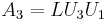$A_3 = L U_3 U_1$ for some upper triangular square matrix $U_1$ with ones on the diagonal ( $U_1$ clears entries of $L U_3$ and adds entries of $A_3$ by way of the upper left corner). Now 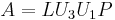$A = L U_3 U_1 P$ is a decomposition of the desired form.

Theoretical complexity

If two matrices of order n can be multiplied in time M(n), where M(n)≥n^a for some a>2, then the LU decomposition can be computed in time O(M(n)).^[3] This means, for example, that an O(n^2.376) algorithm exists based on the Coppersmith–Winograd algorithm.

Small example

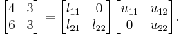
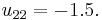
$\begin{bmatrix} 4 & 3 \\ 6 & 3 \\ \end{bmatrix} = \begin{bmatrix} l_{11} & 0 \\ l_{21} & l_{22} \\ \end{bmatrix} \begin{bmatrix} u_{11} & u_{12} \\ 0 & u_{22} \\ \end{bmatrix}.$

One way of finding the LU decomposition of this simple matrix would be to simply solve the linear equations by inspection. You know that:

$l_{11} \cdot u_{11} %2B 0 \cdot 0 = 4$

$l_{11} \cdot u_{12} %2B 0 \cdot u_{22} = 3$

$l_{21}\cdot u_{11} %2B l_{22} \cdot 0 = 6$

$l_{21}\cdot u_{12} %2B l_{22} \cdot u_{22} = 3.$

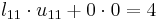
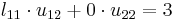
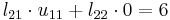
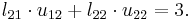
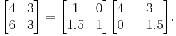
Such a system of equations is underdetermined. In this case any two non-zero elements of L and U matrices are parameters of the solution and can be set arbitrarily to any non-zero value. Therefore to find the unique LU decomposition, it is necessary to put some restriction on L and U matrices. For example, we can require the lower triangular matrix L to be a unit one (i.e. set all the entries of its main diagonal to ones). Then the system of equations has the following solution:

$l_{21} = 1.5$

$u_{11} = 4$

$u_{12} = 3$

$u_{22} = -1.5.$

Substituting these values into the LU decomposition above:

$\begin{bmatrix} 4 & 3 \\ 6 & 3 \\ \end{bmatrix} = \begin{bmatrix} 1 & 0 \\ 1.5 & 1 \\ \end{bmatrix} \begin{bmatrix} 4 & 3 \\ 0 & -1.5 \\ \end{bmatrix}.$

Sparse matrix decomposition

Special algorithms have been developed for factorizing large sparse matrices. These algorithms attempt to find sparse factors L and U. Ideally, the cost of computation is determined by the number of nonzero entries, rather than by the size of the matrix.

These algorithms use the freedom to exchange rows and columns to minimize fill-in (entries which change from an initial zero to a non-zero value during the execution of an algorithm).

General treatment of orderings that minimize fill-in can be addressed using graph theory.

Applications

Solving linear equations

Given a matrix equation

$A x = L U x = b \,$

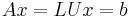
we want to solve the equation for x given A and b. In this case the solution is done in two logical steps:

First, we solve the equation $Ly = b$ for y
Second, we solve the equation $Ux = y$ for x.

Note that in both cases we have triangular matrices (lower and upper) which can be solved directly using forward and backward substitution without using the Gaussian elimination process (however we need this process or equivalent to compute the LU decomposition itself). Thus the LU decomposition is computationally efficient only when we have to solve a matrix equation multiple times for different b; it is faster in this case to do an LU decomposition of the matrix A once and then solve the triangular matrices for the different b, than to use Gaussian elimination each time.

Inverse matrix

When solving systems of equations, b is usually treated as a vector with a length equal to the height of matrix A. Instead of vector b, we have matrix B, where B is an n-by-p matrix, so that we are trying to find a matrix X (also a n-by-p matrix):

$A X = L U X = B.$

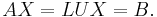
We can use the same algorithm presented earlier to solve for each column of matrix X. Now suppose that B is the identity matrix of size n. It would follow that the result X must be the inverse of A.^[4]

Determinant

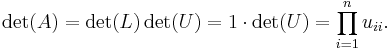
The matrices $L$ and $U$ can be used to compute the determinant of the matrix $A$ very quickly, because det(A) = det(L) det(U) and the determinant of a triangular matrix is simply the product of its diagonal entries. In particular, if L is a unit triangular matrix, then

$\det(A) = \det(L) \det(U) = 1 \cdot \det(U) = \prod_{i=1}^n u_{ii}.$

The same approach can be used for LUP decompositions. The determinant of the permutation matrix P is (−1)^S, where $S$ is the number of row exchanges in the decomposition.

References

^ Poole, David (2006), Linear Algebra: A Modern Introduction (2nd ed.), Canada: Thomson Brooks/Cole, ISBN 0-534-99845-3 .
^ Golub, Gene H.; Van Loan, Charles F. (1996), Matrix Computations (3rd ed.), Baltimore: Johns Hopkins, ISBN 978-0-8018-5414-9 .
^ J.R. Bunch and J.E. Hopcroft, Triangular factorization and inversion by fast matrix multiplication, Mathematics of Computation, 28 (1974) 231–236.
^ Matrix Computations. 3rd Edition, 1996. p121.

Bau III, David; Trefethen, Lloyd N. (1997), Numerical linear algebra, Philadelphia: Society for Industrial and Applied Mathematics, ISBN 978-0-89871-361-9
Cormen, Thomas H.; Leiserson, Charles E.; Rivest, Ronald L.; Stein, Clifford (2001), Introduction to Algorithms, MIT Press and McGraw-Hill, ISBN 978-0-262-03293-3
Horn, Roger A.; Johnson, Charles R. (1985), Matrix Analysis, Cambridge University Press, ISBN 0-521-38632-2 . See Section 3.5.
Householder, Alston (1975), The Theory of Matrices in Numerical Analysis .
Okunev, Pavel; Johnson, Charles (1997), Necessary And Sufficient Conditions For Existence of the LU Factorization of an Arbitrary Matrix, arXiv:math.NA/0506382 .
Press, WH; Teukolsky, SA; Vetterling, WT; Flannery, BP (2007), "Section 2.3", Numerical Recipes: The Art of Scientific Computing (3rd ed.), New York: Cambridge University Press, ISBN 978-0-521-88068-8, http://apps.nrbook.com/empanel/index.html?pg=48

External links

References

LU decomposition on MathWorld.
LU decomposition on Math-Linux.
Module for LU Factorization with Pivoting, Prof. J. H. Mathews, California State University, Fullerton
LU decomposition at Holistic Numerical Methods Institute

Computer code

LAPACK is a collection of FORTRAN subroutines for solving dense linear algebra problems
ALGLIB includes a partial port of the LAPACK to C++, C#, Delphi, etc.
C++ code, Prof. J. Loomis, University of Dayton
C code, Mathematics Source Library
Pseudo-code: Gaussian elimination approach, Prof. P. Wapperom, Virginia Tech
Pseudo-code: Doolittle algorithm, Prof. P. Wapperom, Virginia Tech
LU in X10

Online resources

WebApp descriptively solving systems of linear equations with LU Decomposition
Matrix Calculator, bluebit.gr
LU Decomposition Tool, uni-bonn.de
LU Decomposition by Ed Pegg, Jr., The Wolfram Demonstrations Project, 2007.

Numerical linear algebra

Key concepts	Floating point · Numerical stability · BLAS

Problems	Matrix multiplication · Matrix decompositions · Linear equations · Sparse problems

Hardware	CPU cache · TLB · Cache-oblivious algorithm · SIMD · Multiprocessing

Software	Specialized libraries · General purpose software